
Spreadsheets house massive amounts of data. You can use pivot tables to summarize that data, but what if you want to gain some insight just by glancing at your sheet? Conditional formatting in Google Sheets will give you that insight.
Conditional formatting—which allows you to highlight cells that meet certain criteria—can help you better understand spreadsheets at a glance and create spreadsheets that are more human-readable by your whole team. It also serves as a great way to track goals, giving you visual indications of how you're progressing against specific metrics.
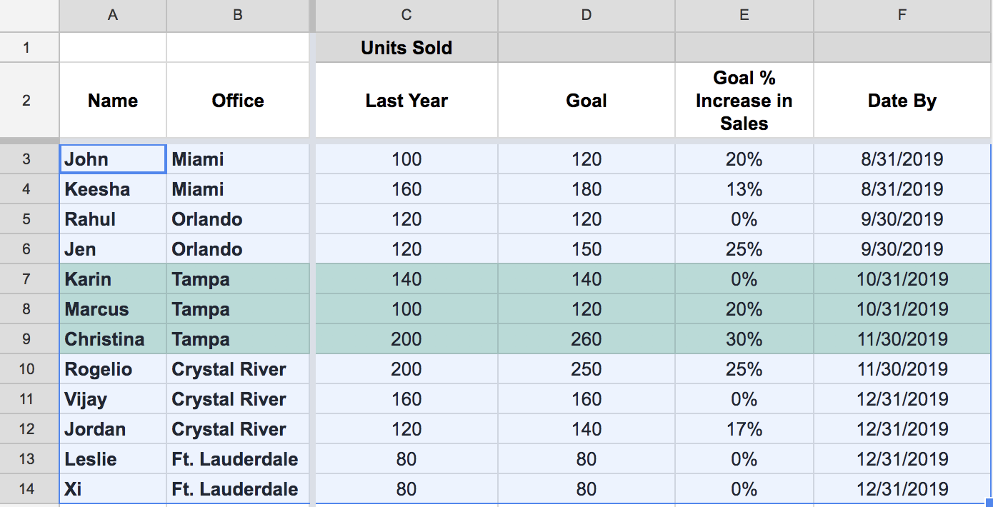
Here, we'll walk through the basics of conditional formatting in Google Sheets. To follow along, use our demo sheet. Open the spreadsheet, select File > Make a copy, and then play around with it as we proceed through the tutorial.
What Is Conditional Formatting?
Google Sheets conditional formatting allows you to change the aspect of a cell—that is, a cell's background color or the style of the cell's text—based on rules you set. Every rule you set is an if/then statement. For example, you might say "If cell B2 is empty, then change that cell's background color to black."
All rules will follow that same structure, so let's define the various elements:
-
Range. Range defines which cell or cells the rule should apply to. In the example above, the range is "cell B2."
-
If cause. What trigger event needs to happen in order for the rule to play out? In the example above, the if cause is "is empty."
-
Style. The rule will play out by changing the style of your cell in whatever capacity you select. In the example above, the style is "background color to black."
How to Use Conditional Formatting in Google Sheets
We'll get into the details below, but here are the basic steps for conditional formatting in Google Sheets:
Step 1: Select a range.
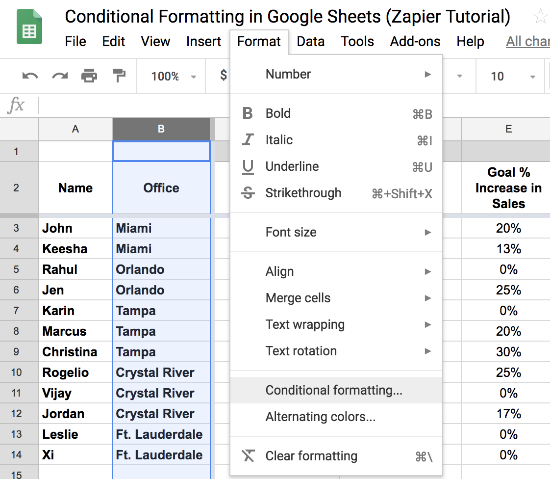
Step 2: Click Format > Conditional Formatting.
Step 3: Select your trigger from the dropdown under Format cells if…
Step 4: Select your formatting style under Formatting style.
Step 5: Click Done.
To learn more specifics and practice with our demo spreadsheet, keep reading.
1. Select a Range
To start using the conditional formatting feature, you have two options.
Option 1: Select a range (cells, columns, or rows) and then click Format > Conditional formatting. This will pop up a conditional formatting toolbar on the right side of your screen. If you're not dealing with too much data, this is the way to go.
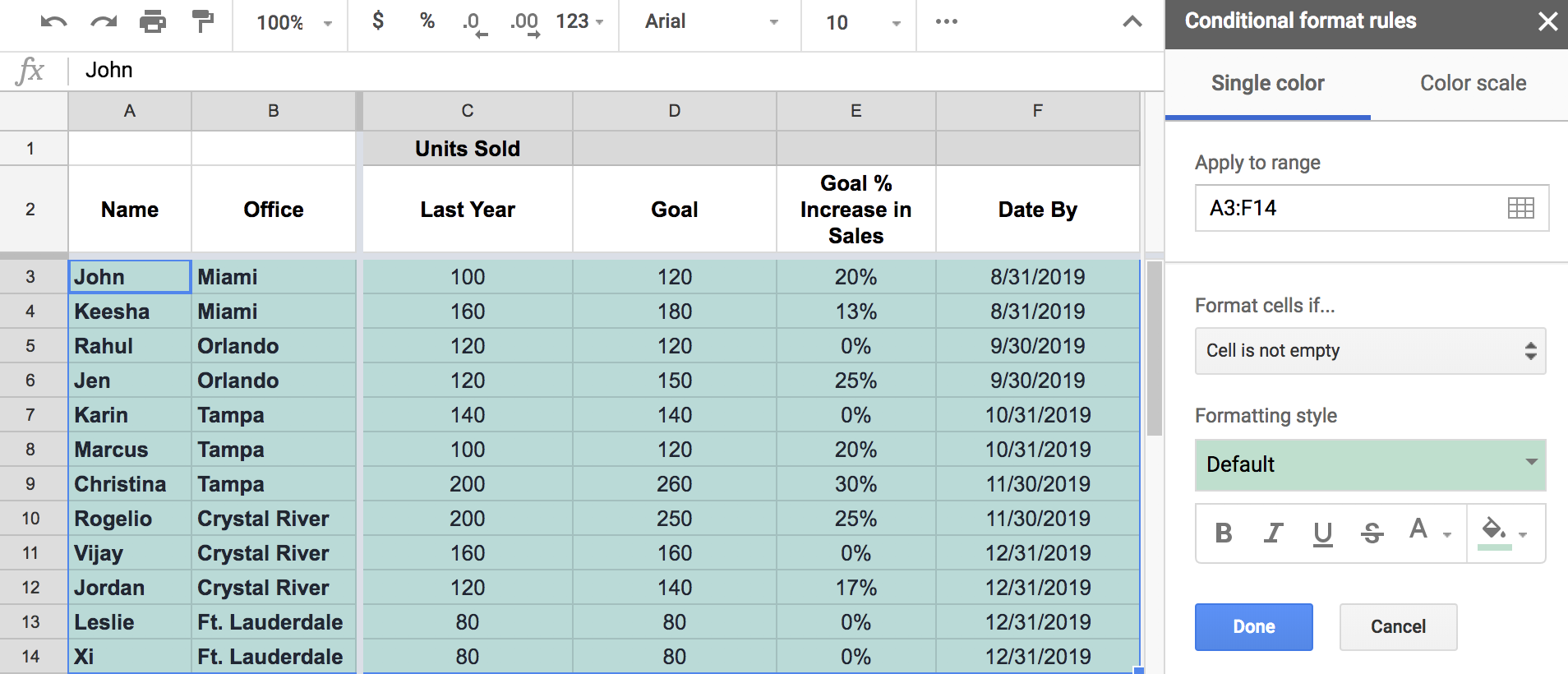
Option 2: If you're working with large amounts of data, click Format > Conditional Formatting right off the bat, and then enter your range under the Apply to range tab.
If you're targeting a single cell, put the tag of the cell there (e.g., A3). If you want to apply your conditional formatting to a larger range of cells, enter the tag of the first and last cell in your desired range, separating them by a colon (e.g., E3:E13).
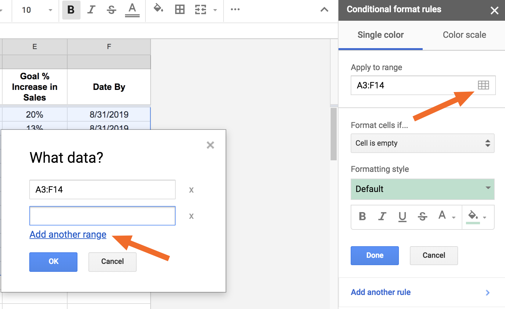
You can add multiple ranges by clicking the icon to the right of the range field and selecting Add another range.
2. Select a Style
It might seem unintuitive to start with the result, but the moment you set your if cause, your cells will change aspect. So it makes sense to set the style first so you can see what the formatting will look like as you go.
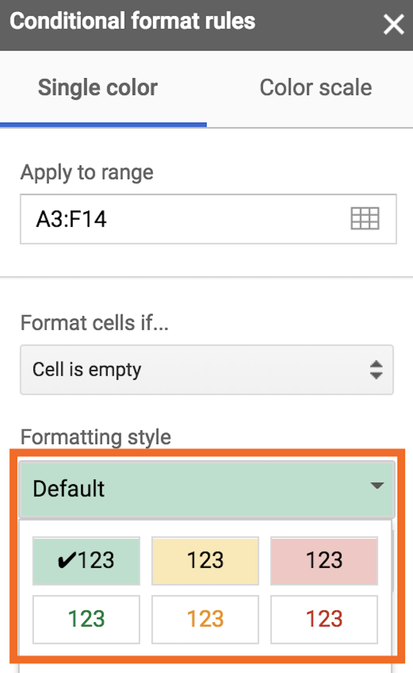
Under Formatting style, click Default, and you'll see the default styling options.
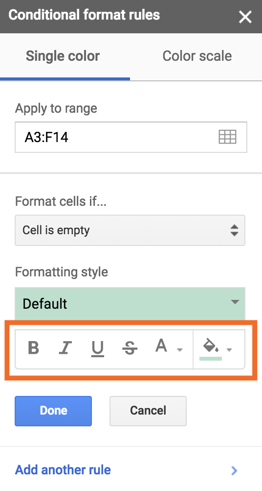
If none of these options are what you're looking for, you can create a custom style, and doing so is no different from selecting your style for anything else in a spreadsheet. You can choose for the text style to be bold, italics, underline, or strikethrough, and you can select your font color and cell background color.
For this demo, we'll be working with the default, which is to turn the background of a cell a seafoam green color, but take some time to play around with the styling to see which colors pop most to you.
3. Create the If Cause
The trigger for a conditional formatting rule can look very different on a case-by-case basis. Let's take a look at a few options.
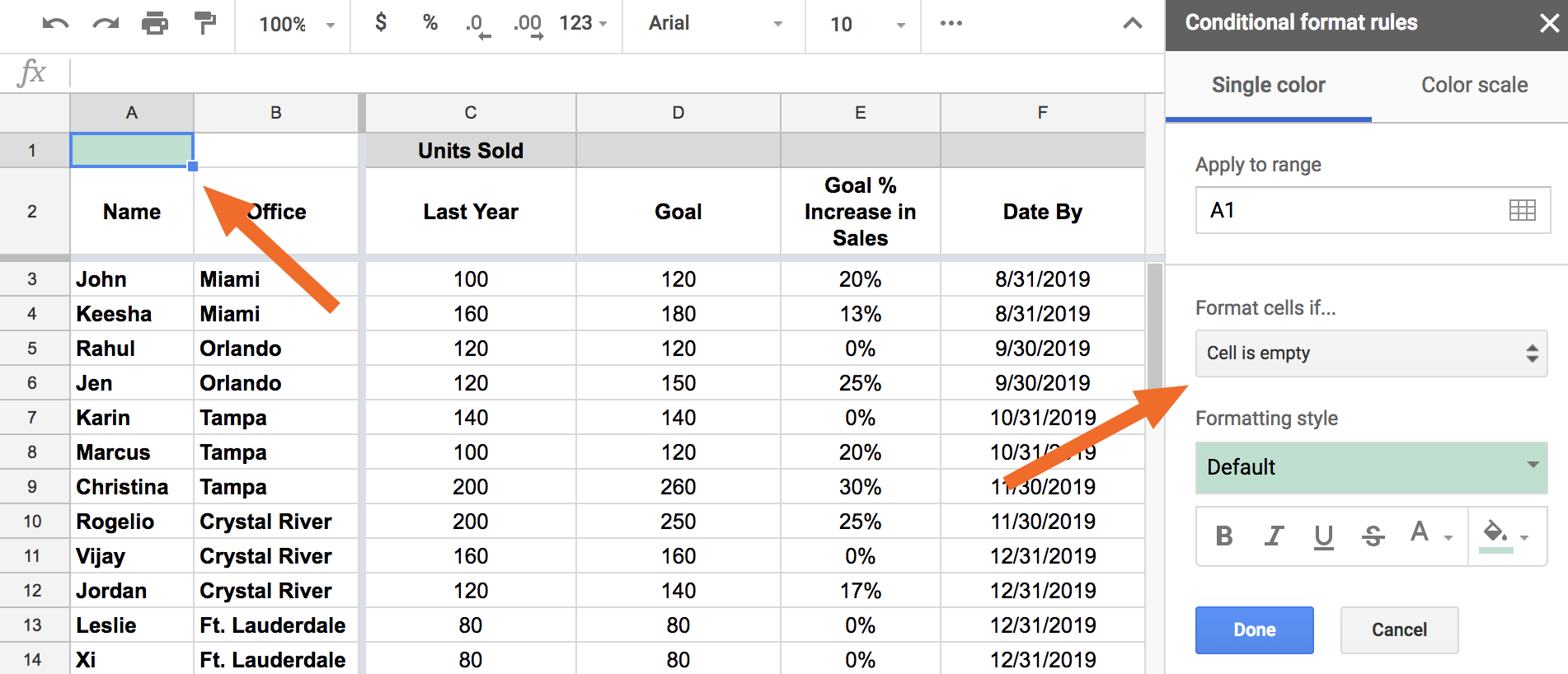
In our demo sheet, select cell A1, and click Format > Conditional Formatting. By default, the if cause (Format cells if…) is set to Cell is not empty, but click it and you'll pull down a whole slew of options.
Let's take a closer look at each option.
Conditional formatting with empty/not empty
The first set of options—Cell is empty and Cell is not empty—will trigger based on whether there's any data in that cell. As an example, select Cell is empty. Because the cell you clicked on (A1) is empty, the default conditional formatting will be applied, and you'll see the cell change color. Magic. (Note: not actually magic.)
Conditional formatting with text
With a text-based rule, a cell will change based on what text you type into it. And you can trigger off of a variety of options:
- Text contains
- Text does not contain
- Text starts with
- Text ends with
- Text is exactly
Let's say you want to highlight all of your reps in Tampa.
Step 1: Select the Office column, column B, and click Format > Conditional formatting.
Step 2: If prompted, click Add new rule.
Step 3: Under Format cells if… select Text contains. Then, where it says Value or formula, type Tampa (not case sensitive).
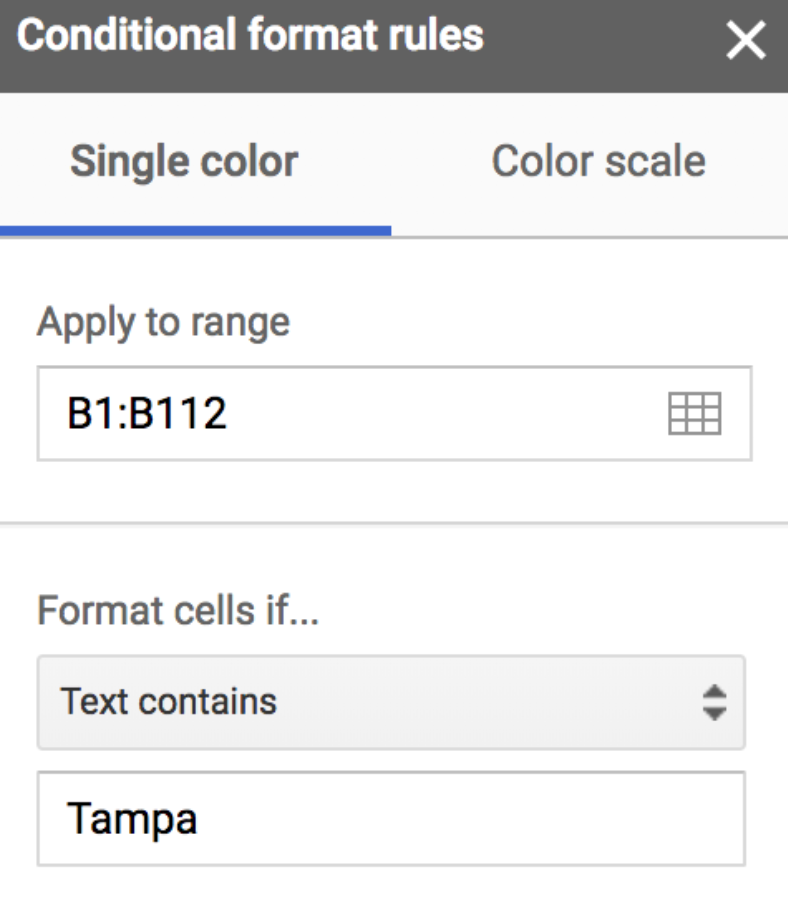
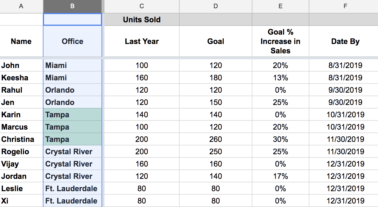
Now, any cell that contains the word Tampa will have the default style applied. And because you highlighted the entire column, any time you add a new rep in the Tampa office, it'll be highlighted for easy access.
Whole Row Conditional Formatting
But let's take it a step further. What if you want to highlight the whole row for any of the Tampa reps? That's where the custom formula option comes in.
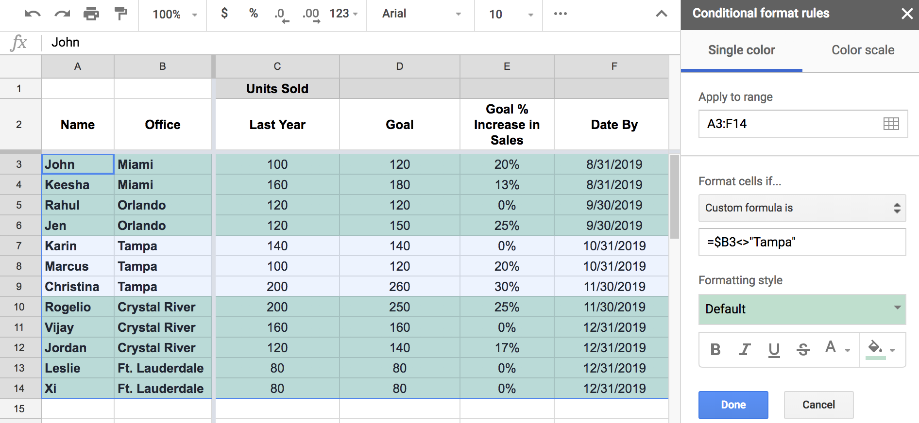
Step 1: Select your entire data set (in this case, A3:F14) and select Format > Conditional formatting. If prompted, select Add new rule.
Step 2: Under Format cells if…, select Custom formula is (all the way at the bottom). You will then be prompted for a value. Type =$B3="Tampa".
Any row that has Tampa in column B will be highlighted.
How did that work? Let's break it down.
The = symbol indicates the start of the formula. The B3 is your sample data for that column: You're indicating that you want Google Sheets to look at column B, but you need to pick a specific cell to do so. The $ before that is what tells Google Sheets to only look at column B. (If you put another $ in front of 3, it would only look at row 3 as well.) And, of course ="Tampa" tells Google Sheets what text to look for.
You can do the same thing if you want to highlight any rows that don't include a given value. Maybe you want to highlight any reps who don't work out of Tampa, for example. To do that, you'll change that second = to <>, so it looks like this: =$B3<>"Tampa".
Of course, the Custom formula feature can be used for a whole variety of cases. You can refer to a list of formulas accepted by Google Sheets, but be warned: They get advanced pretty quickly.
Conditional formatting with numbers
If you want to trigger conditional formatting based on numbers, you have eight options:
- Greater than
- Greater than or equal to
- Less than
- Less than or equal to
- Is equal to
- Is not equal to
- Is between
- Is not between
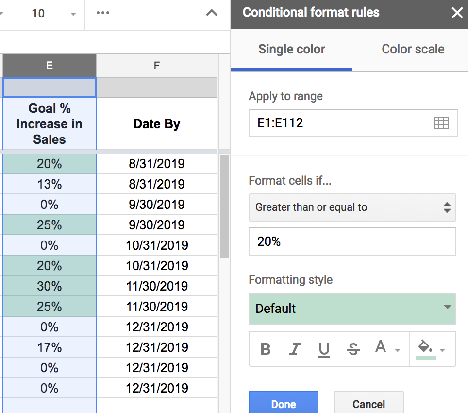
On the demo spreadsheet, let's say you want to highlight any stretch goals: cells where the goal increase is 20% or higher.
Step 1: Highlight the "Goal % Increase in Sales" column, column E, and select Format > Conditional Formatting > Add new rule > Greater than or equal to.
Step 2: Type 20% into the field provided.
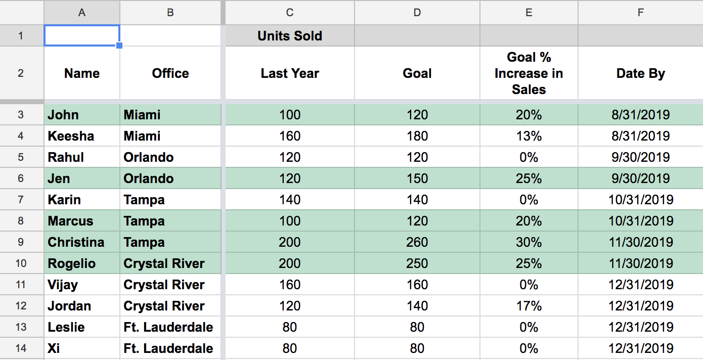
You can apply the whole row formatting to numbers as well. Again, change the range to cover all of the data (A3:F14). Then, under Format cells if… > Custom formula is, type =$E3>=20%.
Now any row where the value in column E is greater than or equal to 20% will be highlighted.
You can play around with the operators to make less than or equal to (<=), less than (<), greater than (>), or equal to (=).
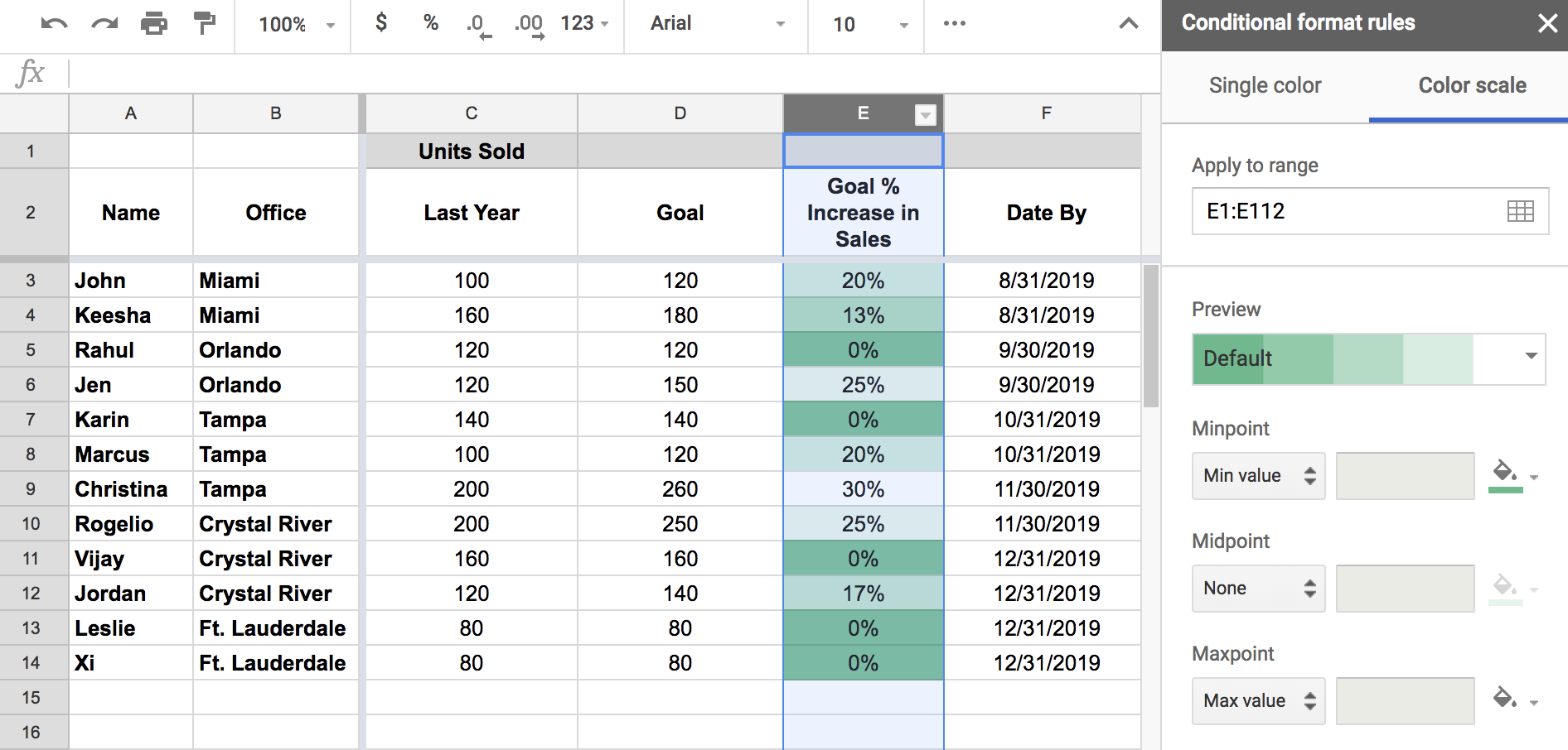
Conditional formatting with a color scale
What if you want to see where each goal falls on a spectrum? With a color scale rule in place, you'll have a basic color applied to a range of cells, but the color will differ in intensity based on the value entered.
In our demo sheet, highlight column E, select Format > Conditional formatting, then click on the Color Scale tab in the conditional formatting toolbar. The default formatting will appear, highlighting the lowest percentages with the most intensity.
Conditional formatting with dates
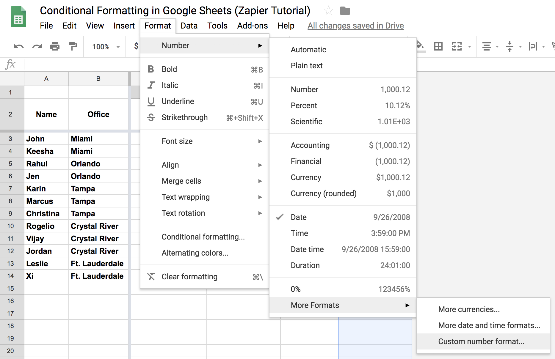
Before we dive into using conditional formatting with dates, it's important to settle on a clear date format. Select any columns that include dates, click Format > Number, and select the style you like. You can select More Formats > Custom number format if you want something that's not listed. It doesn't matter which you choose—whatever is easiest for you to read—but just be sure you're consistent with your formatting.
For date-based conditional formatting, you have three options:
- Date is
- Date is before
- Date is after
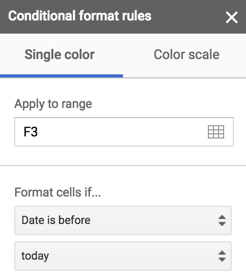
Let's take a look at what we find to be the most useful case for conditional formatting with dates: Date is after today. What this will do is highlight any cell whose date is in the past—that way, you can easily keep track of deadlines.
In our demo sheet, we have a "Date By" column (column F), which is the date by which each employee is supposed to have increased their sales by the percentage in column D. To see it in action, change the date in one of the cells to yesterday's date. Then, select that cell, click Formatting > Conditional Formatting > Date is before > Today.
You should see the cell change color. In addition to relative dates (today, tomorrow, yesterday, in the past week/month/year), you can also use conditional formatting based on an exact date.
Just be sure that you type the date in the exact format you have it in the spreadsheet (e.g., MM/DD/YYYY).
Now that you understand the basics of conditional formatting, take our demo sheet and play around with it. You'll likely find dozens of use cases for conditional formatting to better communicate goals, deadlines, and more with your team.
source https://zapier.com/blog/conditional-formatting-google-sheets/
No comments:
Post a Comment