How to Use Pivot Tables in Google Sheets

Spreadsheets offer powerful analysis capabilities, but sometimes it feels like they're missing that extra layer of insight. When there's a massive amount of data, it's tough to summarize or draw conclusions from a basic tabular spreadsheet view.

Enter: the pivot table.

Most Excel power users employ pivot tables as their bread and butter, but Google Sheets offers the same tool, so you can use pivot tables while keeping things in G Suite. In this article, we'll walk through how to build pivot tables in Google Sheets.

What Are Pivot Tables?

In its simplest form, a spreadsheet is just a set of columns and rows. When a column and a row meet, cells are formed. You can use formulas to log data within these cells—and when your spreadsheet is small, it's simple enough to read through and understand the numbers.

But as your spreadsheet begins to grow, drawing conclusions requires a bit more power. That's where pivot tables come in. A pivot table takes a large set of data and summarizes it.

Think of it this way: Normal spreadsheets essentially have "flat data" represented by two axes, horizontal (columns) and vertical (rows):

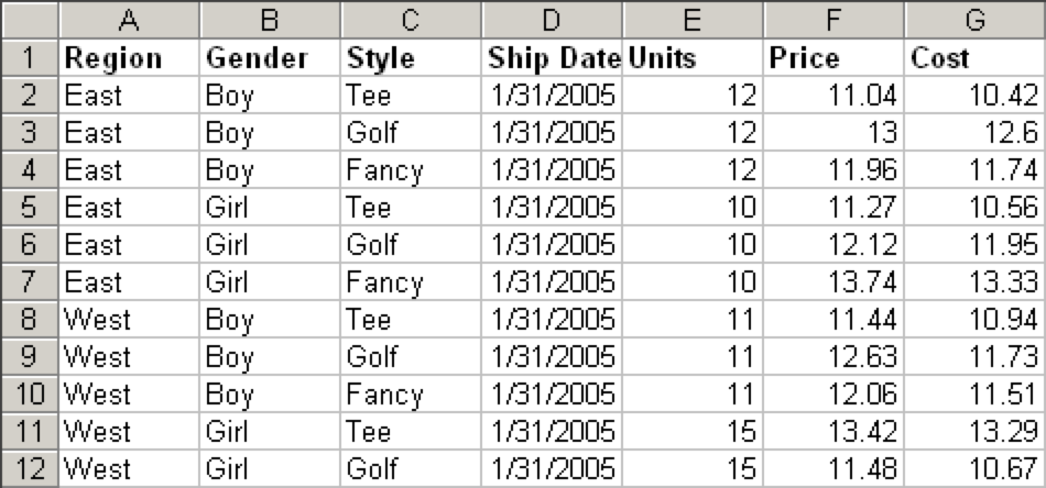
To derive more insights, you'll need to add data on another level. In the case above, for example, you start with each sale as its own row, and each column offers different information about that sale. But if you shift (or pivot) the axes of the table, you can add another dimension:

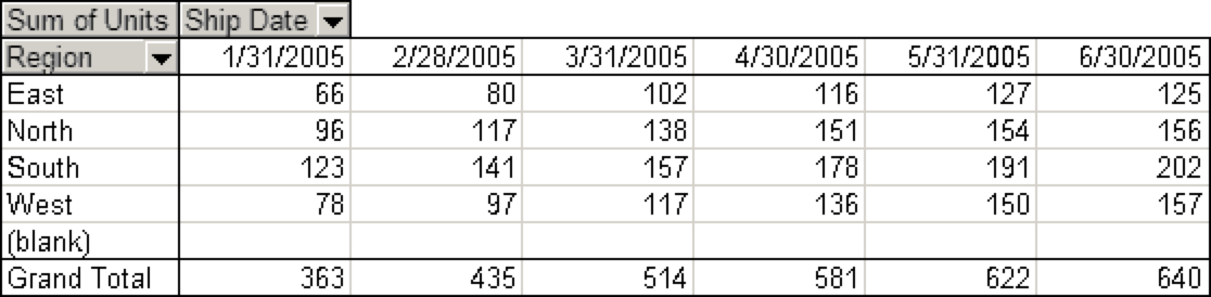
Now, you're not looking at things by individual sale. Instead, you're looking at aggregated data: How many Units did we sell in each Region for every Ship Date?

So that's the rough idea: You can take a two-dimensional table and pivot it around an aggregation of the data to introduce a third dimension. And that's how you get a pivot table. Doing so helps you see the bird's eye view, derive meaning from large quantities of data, and surface unique insights.

While you could derive many of these insights using formulas, the pivot table allows you to distill it in a fraction of the time—and with less chance for human error. Plus, every time your boss asks for a new report based on the same data set, you can generate it with a few clicks, instead of starting from scratch.

How to Use Pivot Tables in Google Sheets

Google Sheets pivot tables are as easy to use as they are powerful. Here's a quick look at how to use them, followed by a more in-depth tutorial.

1. Open a Google Sheets spreadsheet, and select all of the cells containing data.
2. Click Data > Pivot Table.
3. Check if Google's suggested pivot table analyses answer your questions.
4. To create a customized pivot table, click Add next to Rows and Columns to select the data you'd like to analyze.
5. Click Add next to Values to select the values you want to display within the rows and columns.
6. Click Filters to display only values meeting certain criteria.

For this tutorial, we've created a Google Sheets spreadsheet with dummy data. Open the Google Sheet, and select File > Make a copy…, and then follow along with our detailed tutorial below.

Create the pivot table

You have a sheet filled with raw data, so the first thing to do is turn it into a pivot table.

Select all of the cells containing data (command or ctrl + A is a handy shortcut). Then click Data > Pivot Table…, as shown below.

If you're using a data set in which some or all of your columns don't have a name (i.e., the top most row is blank), you'll need to name these columns in order to create a pivot table on this data set.

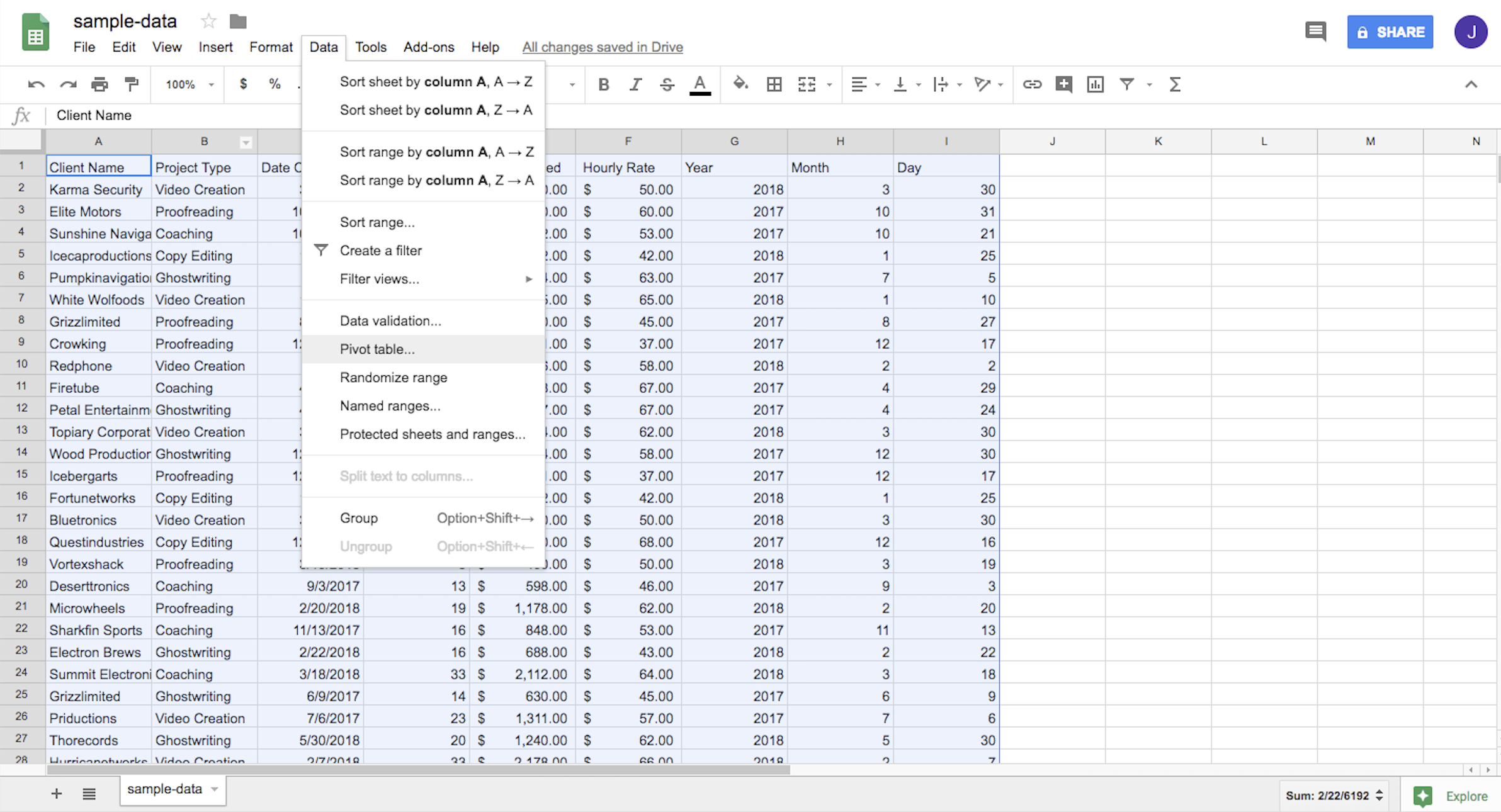
This will create a new sheet on your spreadsheet called "Pivot Table." And that's where you'll be working from.

Learn the pivot table editor

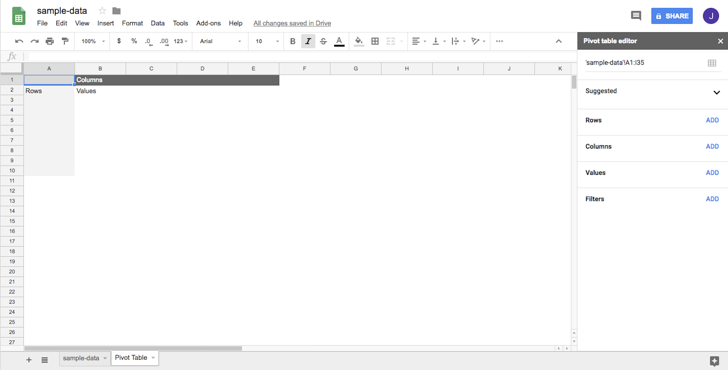
With your pivot table generated, you're ready to start doing some analysis. To do so, you'll use the pivot table editor to build different views of your data. You'll see the editor on the right-hand side of your Google Sheets spreadsheet.

The editor offers two ways to analyze: using Google's suggestions or choosing your dimensions manually.

Suggested pivot tables

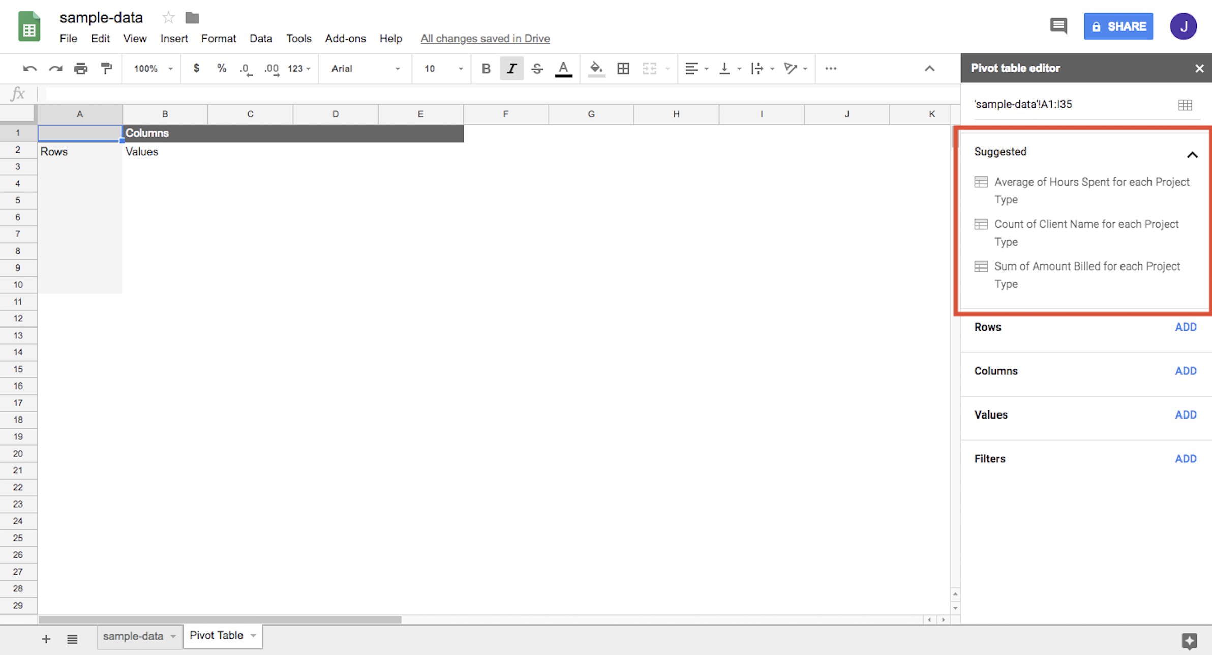
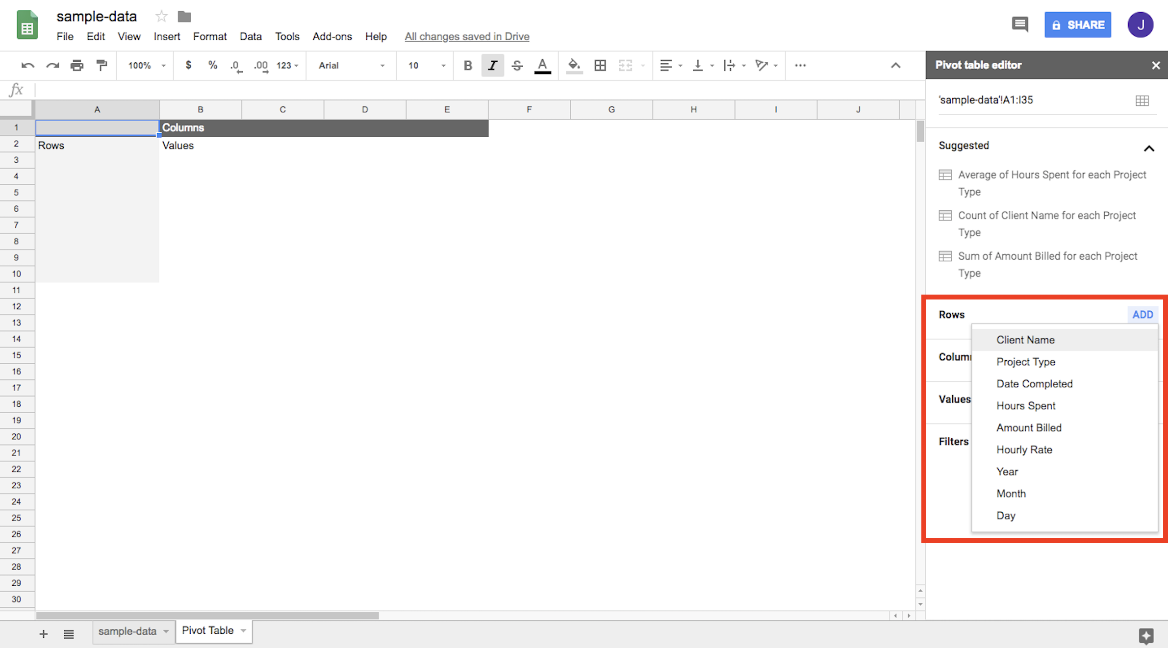
Google being Google, it knows what you want to know before you even know you want to know it. Under "Suggested" in the editor, Google offers analyses for your data set.

For example, given our data set example, it suggests the following analyses:

• Average of Hours Spent for each Project Type
• Count of Client Name for each Project Type
• Sum of Amount Billed for each Project Type

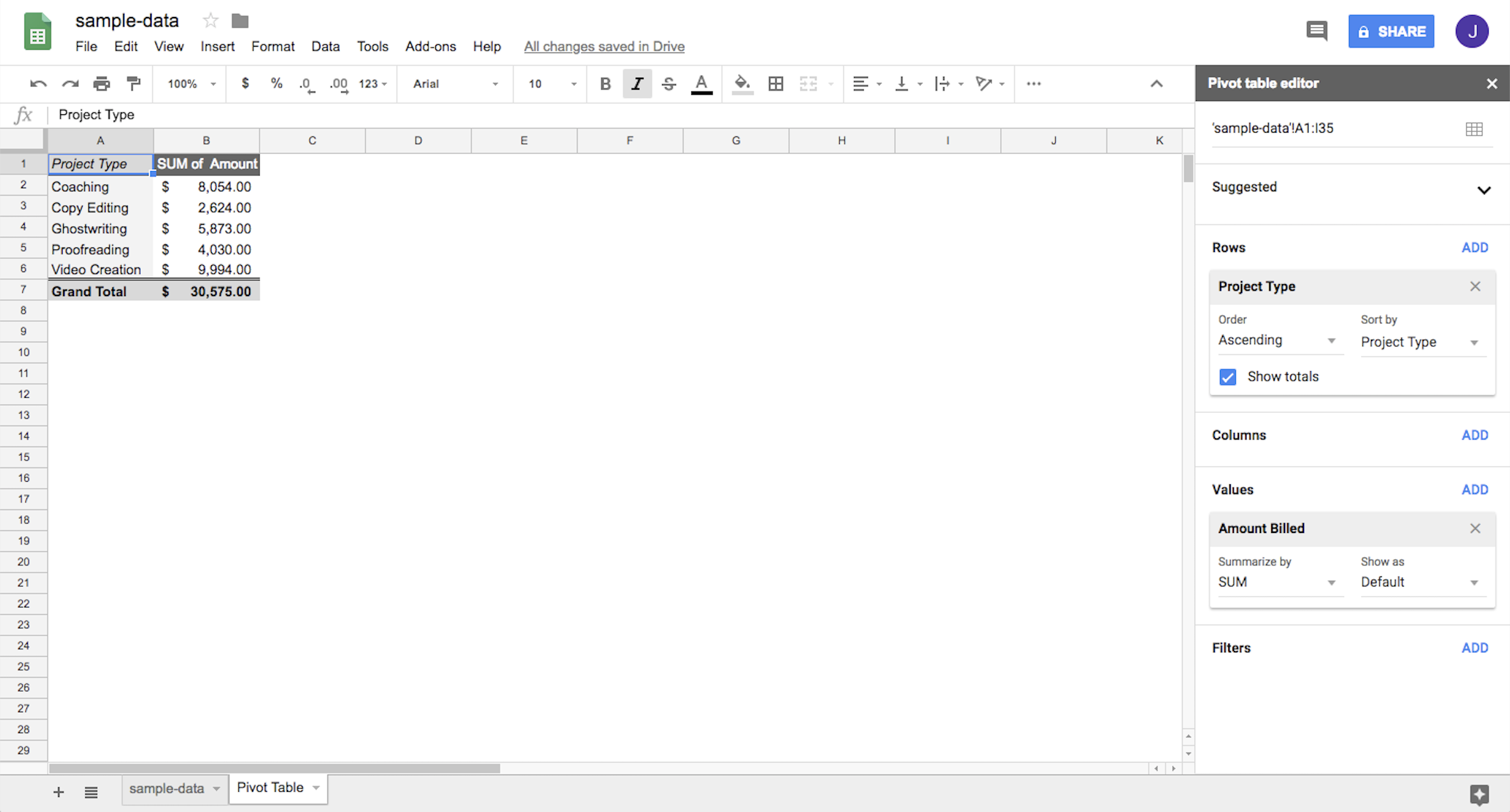
If you click on any of the suggested options, Google Sheets will automatically build out your initial pivot table. For example, click the third option ("Sum of Amount Billed for each Project Type"), and you'll see the project types in Column A and a total amount billed for each in Column B.

Manual options

If the suggested analysis isn't what you're looking for—or if you'd like to perform a different type of analysis—you can manually build your preferred output.

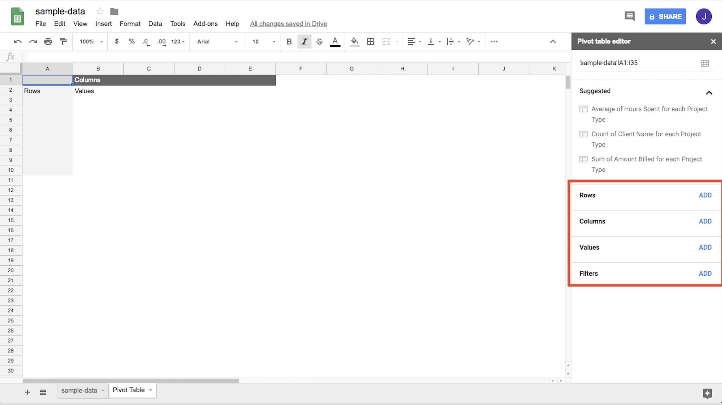
You'll find four options on the right side of your sheet that allow you to insert data into your pivot table:

• Rows
• Columns
• Values
• Filter

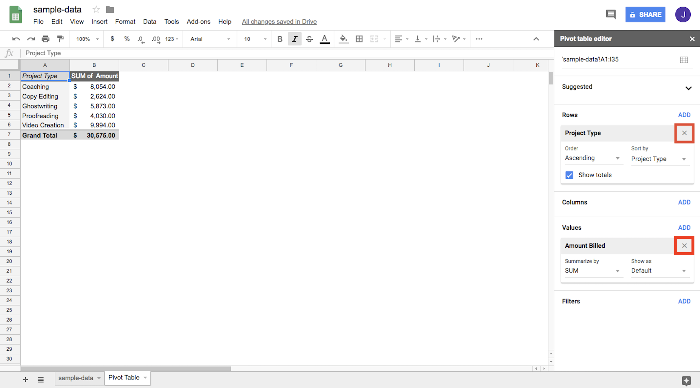
These are the various dimensions you can use to analyze your data. We'll walk through an example analysis to show you how to use them, but first, start by removing the existing selections (created by the suggested analysis we just performed) by clicking X for the Rows and Values options.

You should now be back to your original empty pivot table that you started off with. Here's the analysis we're looking to do:

For each of our clients, across different project types, how much did we bill in 2017?

In this case, we're looking for four things:

• For each client
• Across project types
• Total amount billed
• In 2017

As you night guess, each of those for pieces lines up with one of our elements: rows, columns, values, and filters.

• Rows and columns help you build out the the two-dimensional data set on which you can calculate your third dimension values. In this instance, our base data is Client Name (row) and Project Type (column).

• The value we want to get in the cells where Client Name and Project Type meet is Total Amount Billed.

• How do we show data from only 2017? That's where the filter comes in. The filter allows you to analyze only a specific subset of data.

Click on "Add" for any one of those four options, and you'll get a dropdown with the column names from your original data sheet. If you click on one of those column names, the data will be added in the given format.

Build the report

Now let's get to actually building this thing. Remember, here's the question we're asking:

For each of our clients, across different project types, how much did we bill in 2017?

Step 1: Add rows

First, we need to set up our table to have both the list of clients and project types. Click on Add next to Rows, and select the Client Name column to pull data from.

As the selections imply, you'll now see all your clients' names as rows in your pivot table.

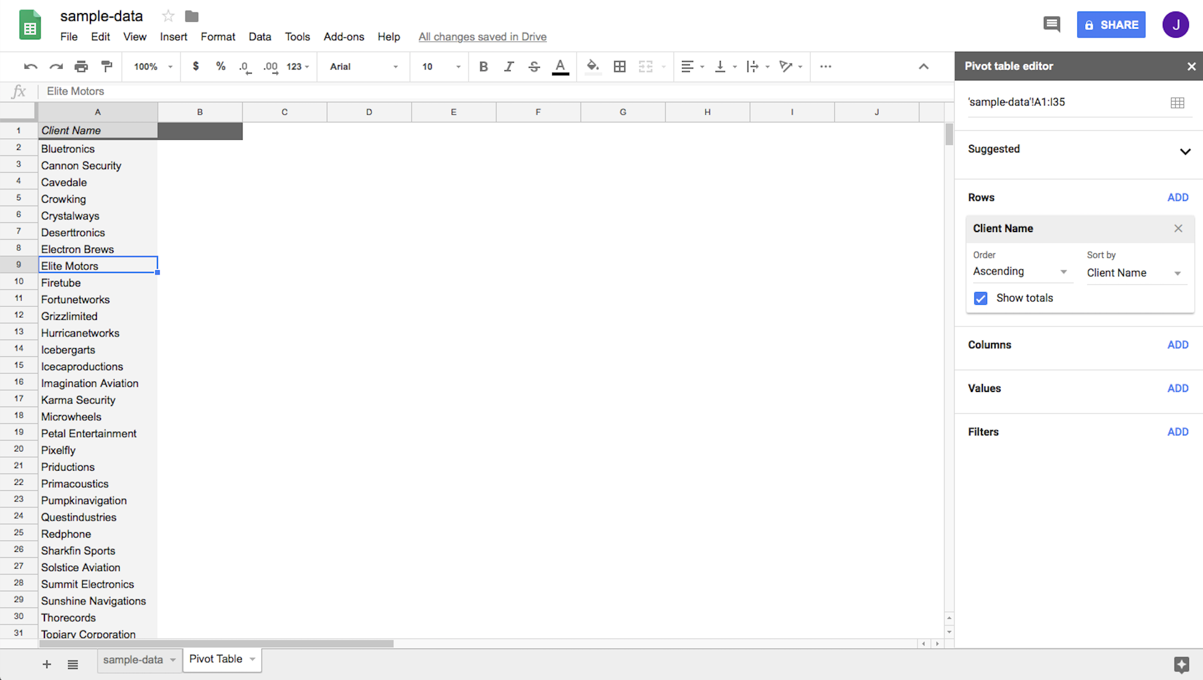
It took the selected portion of the original data, removed any duplicates, and it's now showing you the data in an easy-to-digest report. Column A now has a unique list of clients in alphabetical order (A-Z) by default.

Of course, all you've done so far is add an existing column into your pivot table. You'll need to add more data if you really want to get value from your report.

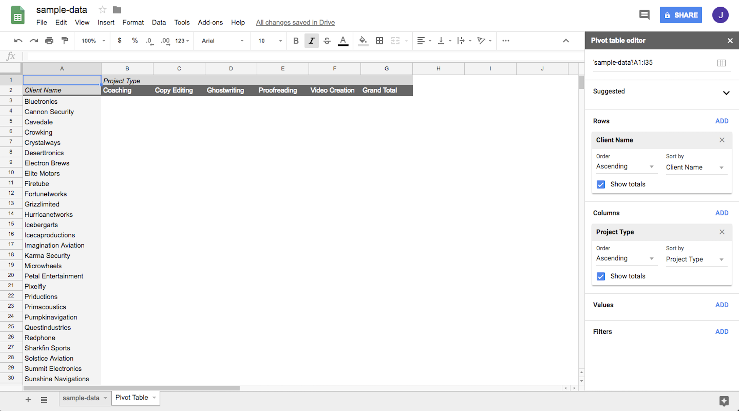
Step 2: Add columns

The next step is adding Project Type as the columns. In the pivot table editor, click on Add next to Columns, and select Project Type. Here's the result:

Step 3: Add values

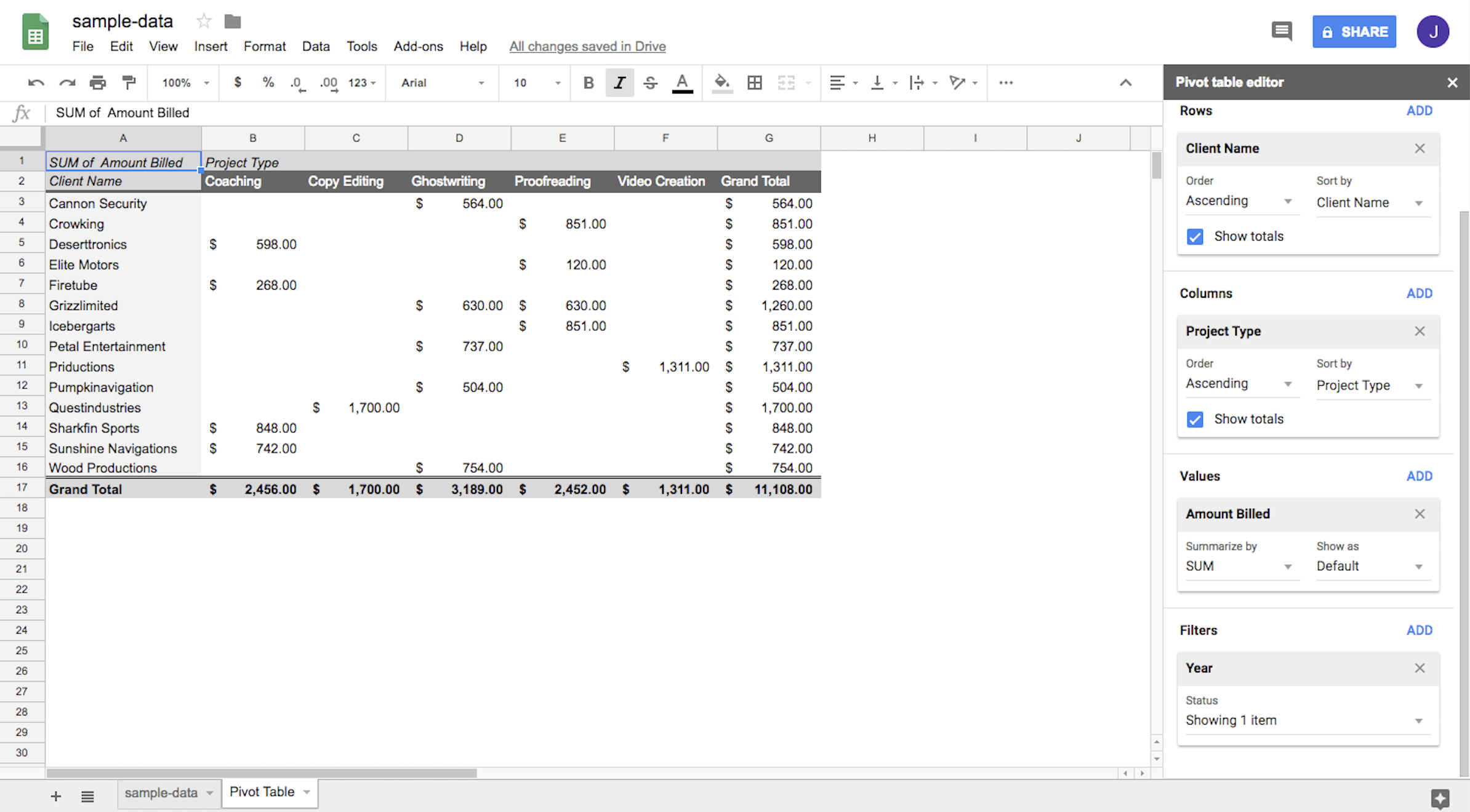
Now that we have our rows and columns, we'll need to bring in calculated values for each individual cell in the pivot table to see total amount billed. In the pivot table editor, click Add next to Values, and select Amount Billed.

To ensure you're seeing a total amount billed (versus, for example, the average amount billed), you'll head to the Summarize by field and select SUM.

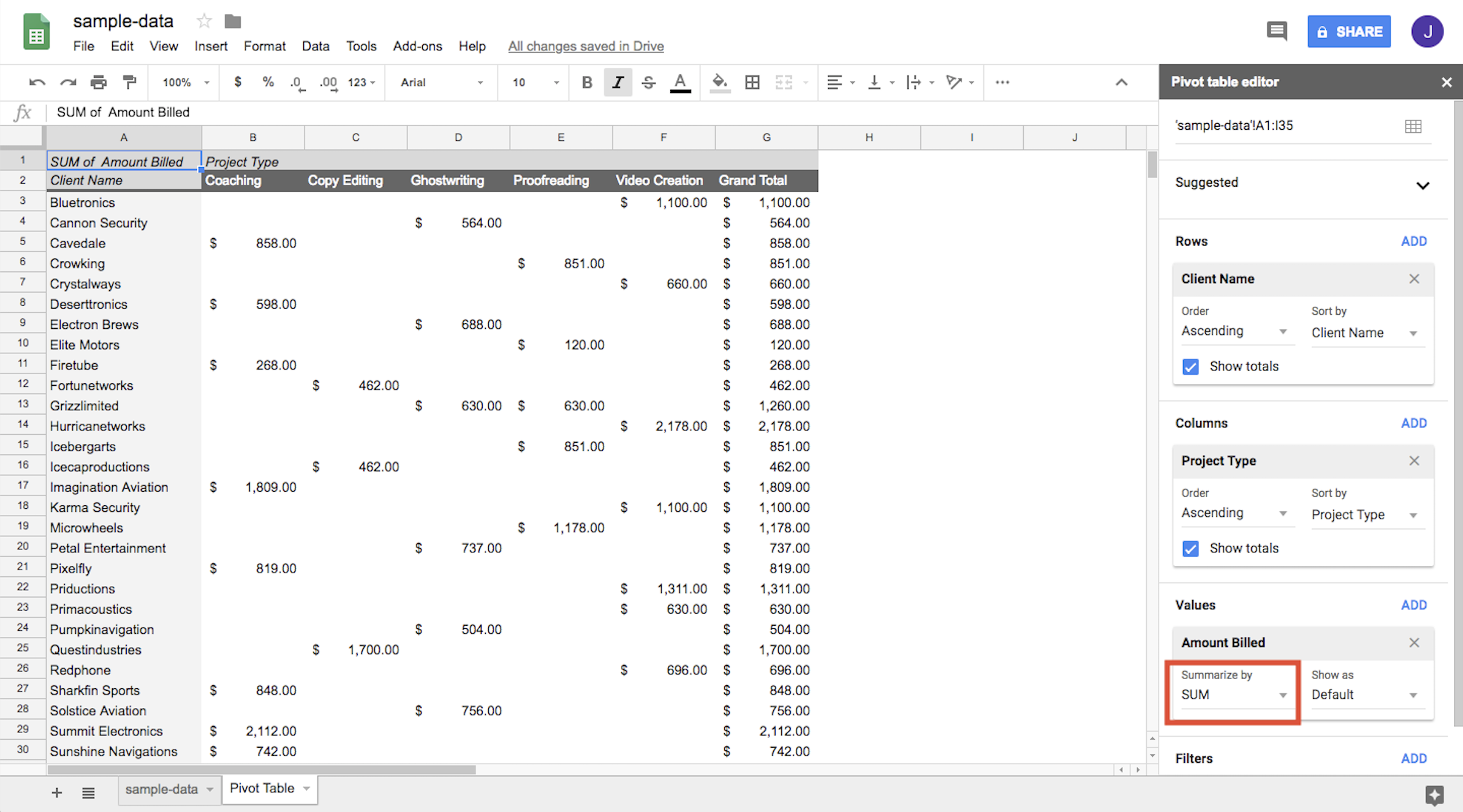
Now we have some useable information: the total amount billed for each type of project we've completed for a given client.

You'll also see that the "Grand Total" is added and calculated automatically. That allows us to see the total amount that we've billed to each client and the total amount that we've billed for a given project type across all clients.

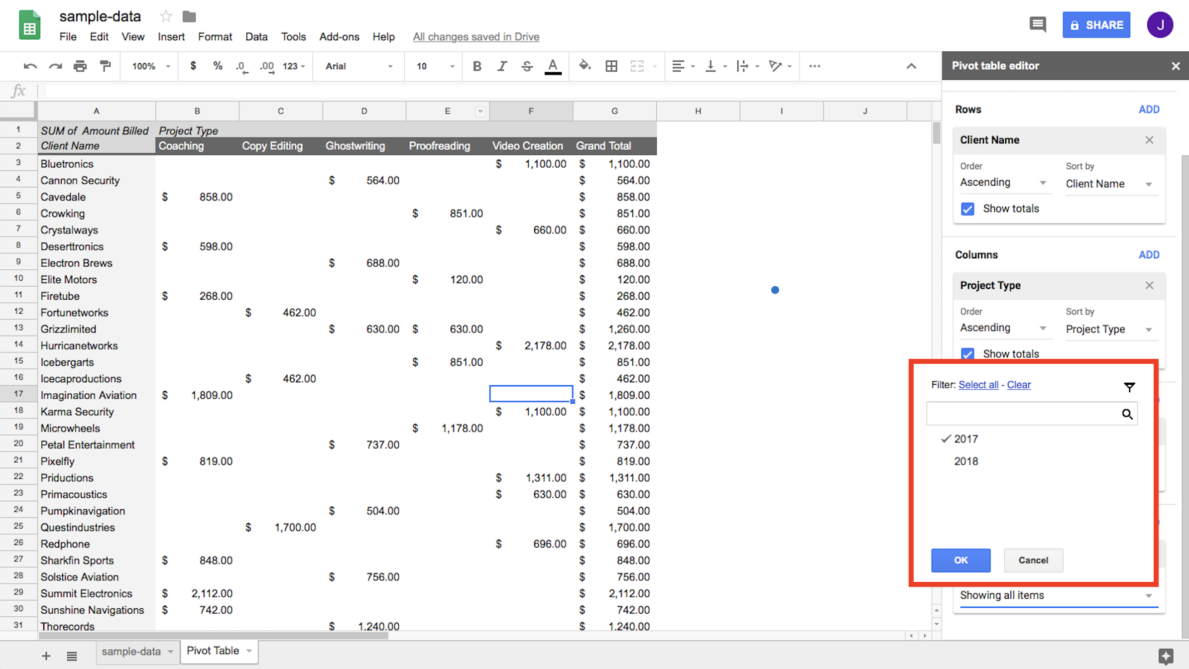
Step 4: Add filters

You can already see the power of the pivot table, but what we've created still doesn't answer our question: we still haven't filtered the table to only show values for 2017.

To do this, click Add next to the Filters option, and select Year. Both 2017 and 2018 (the two years in our original data set) will default to checked. Unselect 2018 and click OK to update the table so it only shows data from 2017.

And that's that. You now have a pivot table table answering the question:

For each of our clients, across different project types, how much did we bill in 2017?

Note: You can filter data based on any column in your original data set.

Read the pivot table

With all of the information we want right in front of us, we can now answer almost any question we have about the data. To solidify our understanding of using pivot tables in Google Sheets, we'll walk through two more examples.

Which client did we bill the most in 2017?

To answer this question, we'll need to simplify our report: We just need the names of our clients as rows and the sum of the amount billed to them as values.

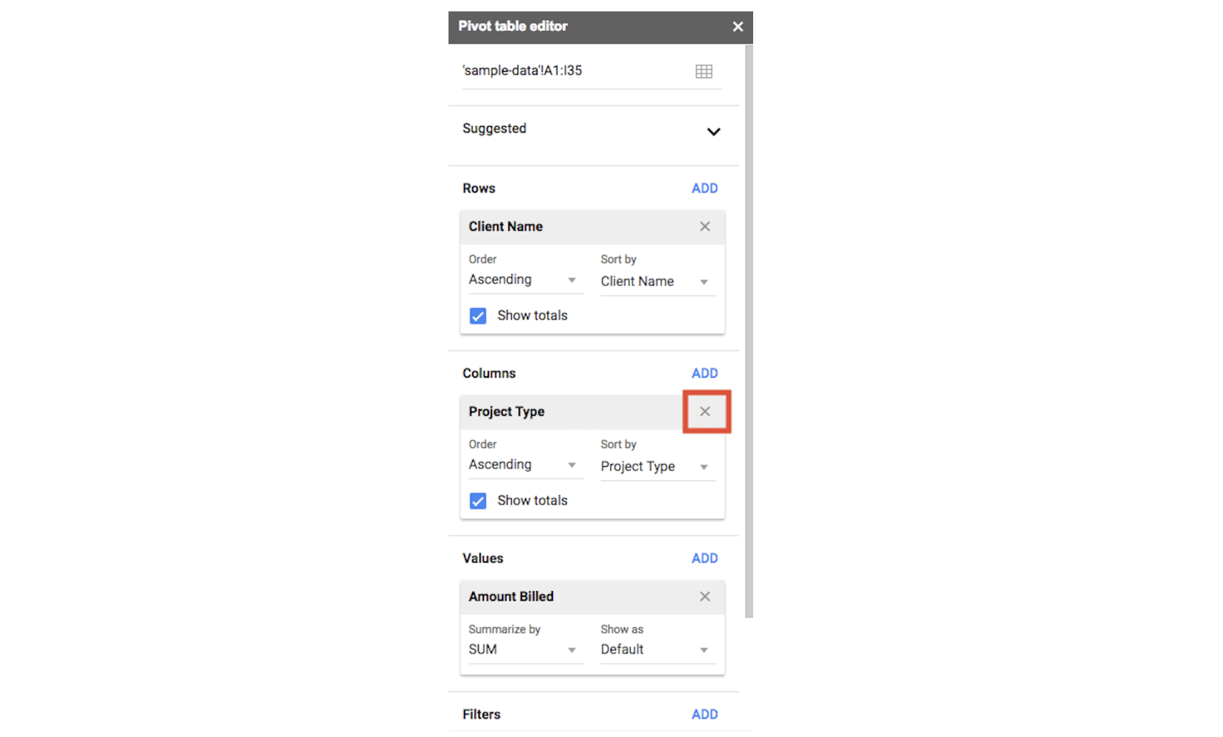
First, you'll need to remove Project Type from the columns by clicking the top right X in the Columns section next to Project Type.

Next, under Client Name, select Sort by > SUM of amount billed, and the table will reorder itself to show you the data in ascending order.

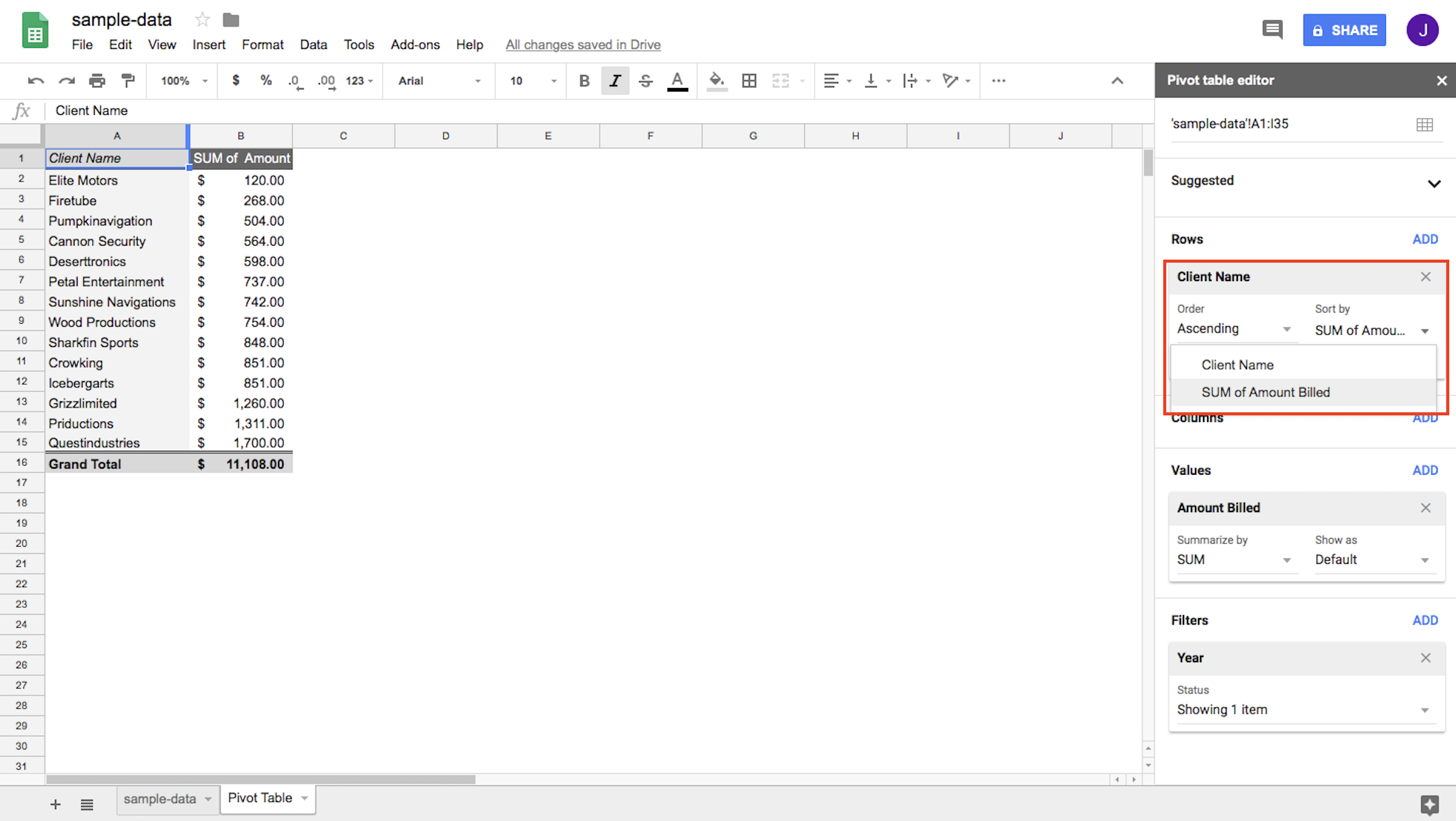
Now we can answer our question: We billed sample company "Questindustries" the most in 2017, at $1,700.

Which project type had the highest hourly rate on average?

Here, we're going to shift our analysis from looking at the total amount billed to the highest average hourly rate for each project type.

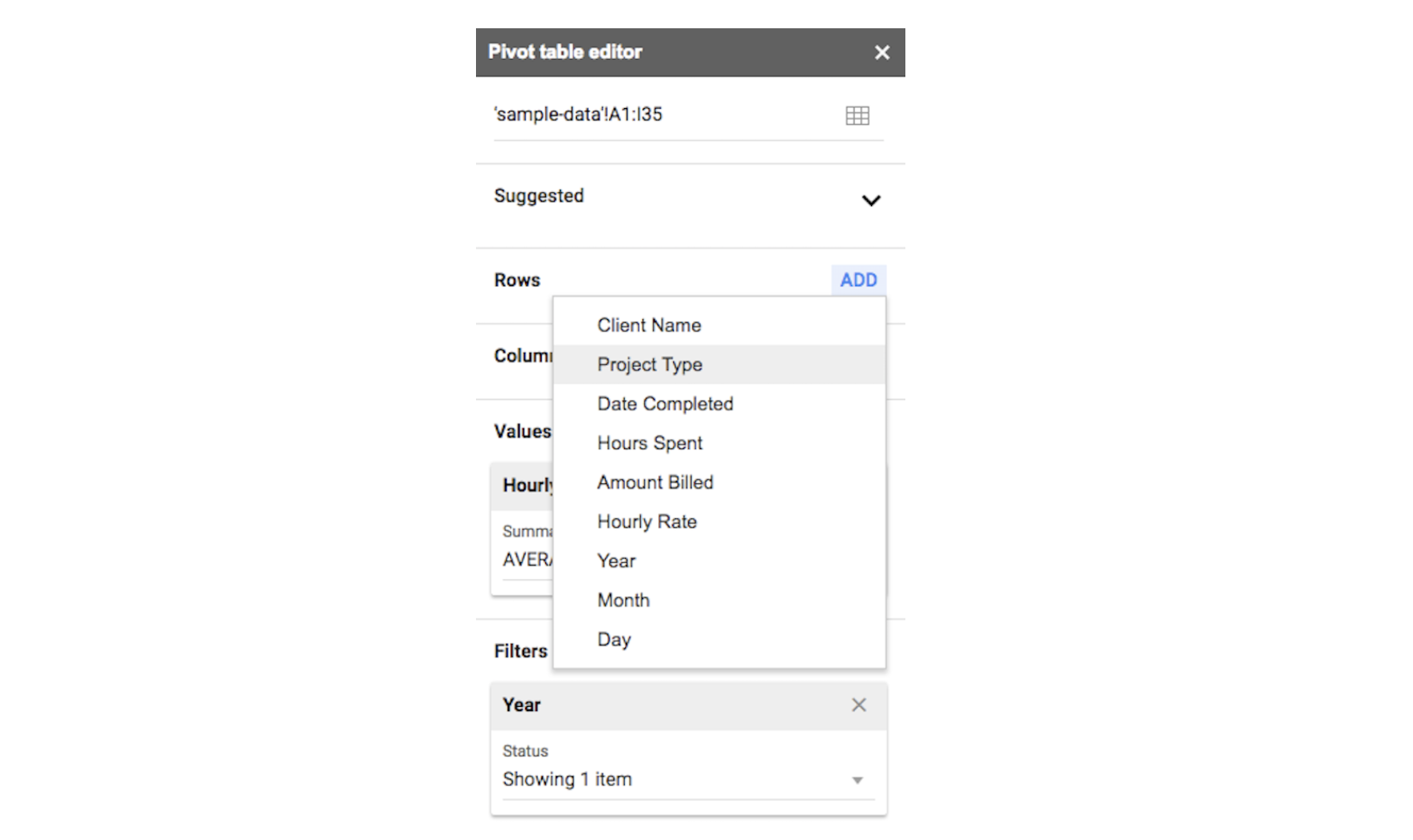
To do this, trade out Client Name for Project Type in the Rows section by clicking the top right X to clear your selection. Then select Project Type as your new rows value.

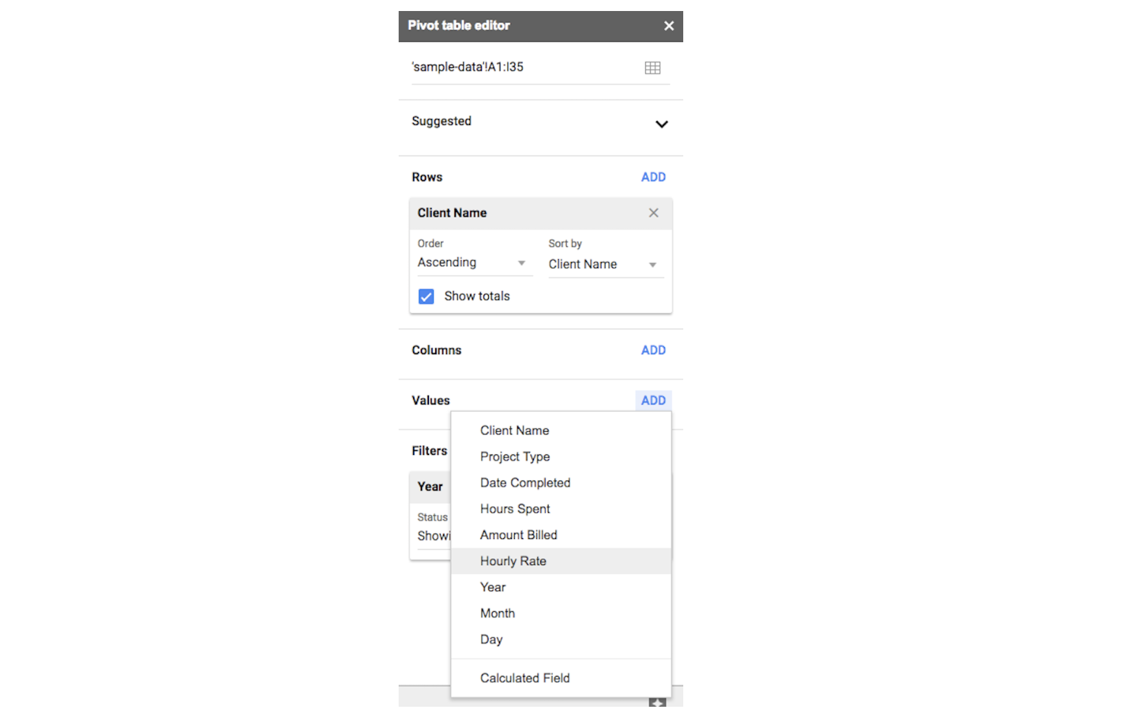
Then, in the Values section, remove Amount Billed and select Hourly Rate instead.

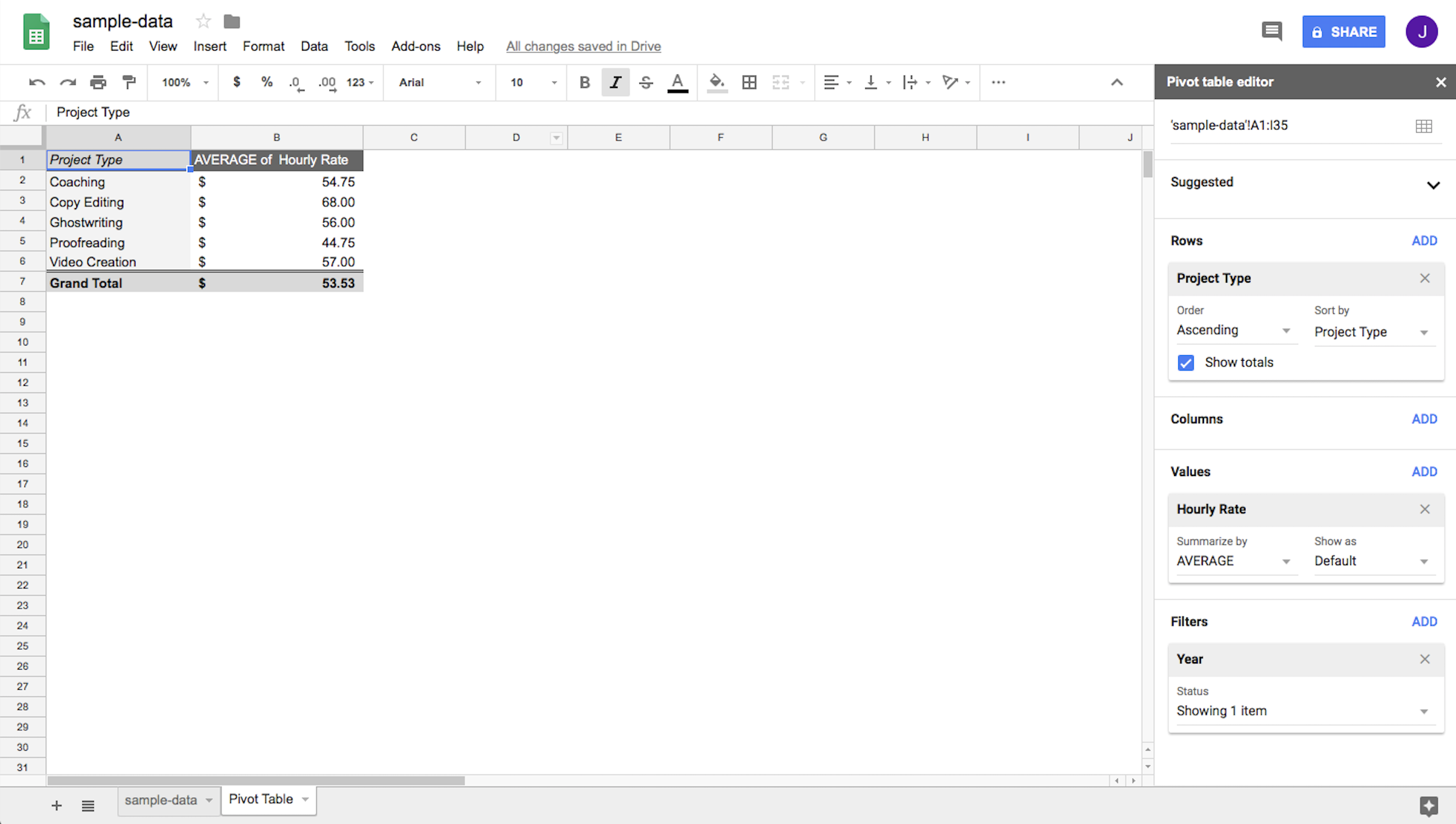
Then change the Values setting from SUM to AVERAGE in order to see the average amount billed, not the sum. You'll see that the highest average hourly rate we charged in 2017 was $68.00 for Copy Editing.

---

Why Use Google Sheets for Pivot Tables?

Zapier helps you get all of your company's data into Google Sheets without lifting a finger. Once you have all that data in one place, you need to analyze it—and now you can do that efficiently using pivot tables. With pivot tables in Google Sheets, you can unlock the potential of your data and distill the information for all stakeholders without using complicated formulas.

Once you've mastered the basics, try taking things to the next level. Use our sample spreadsheet to see what kinds of insights you can find with just a few clicks.

Related Reading:

• How to Automate Google Sheets With Macros—No Coding Required
• How to Find Records Automatically in Google Sheets, Excel, and Zapier
• How to Remove Duplicates in Google Sheets

source https://zapier.com/blog/google-sheets-pivot-table/